![]()
A common approach to causal inference on observational data with continuous treatments is matching, where observations are paired based on covariate similarity while ensuring treatment values are distinct within pairs. Matching allows for estimation of an average treatment effect while adjusting for observed confounding. Inexact covariate matching is common in practice, but may induce severe bias in downstream causal inference. We propose matching, estimation, and inference methods for paired observational studies with continuous treatments that addresses bias caused by inexact covariate matching. The nbpInference package includes methods for calipered non-bipartite matching, bias-corrected sample average treatment effect estimation, and covariate-adjusted conservative variance estimation based on the methods in (Frazier, Heng, and Zhou 2024).
You can install the development version of nbpInference from Github like so:
# install.packages("devtools")
# devtools::install_github("AnthonyFrazierCSU/nbpInference")Below is an example of generating data, forming matched pairs, estimating treatment effects and creating Wald-type confidence intervals for the sample average treatment effect using different functionality in nbpInference. First, we simulate some covariates \(X=(X_1,...,X_5)\), a continuous treatment \(Z\) and outcome \(Y\) based on the data generation models described in the main simulation of (Frazier, Heng, and Zhou 2024).
library(nbpInference)
library(ggplot2)
#> Warning: package 'ggplot2' was built under R version 4.3.3
set.seed(12345)

# generating X, Y, Z with a sample size of 100
example_data <- generate.data.dose(100)

# several rows as an example of data generated
head(example_data)
#>             Z         Y         X1         X2         X3          X4
#> 1  1.45275168 -3.302435  0.5855288  0.2239254 -1.4361457  0.52228217
#> 2  0.58768423  4.525210  0.7094660 -1.1562233 -0.6292596  0.00979376
#> 3  0.91140199  1.579223 -0.1093033  0.4224185  0.2435218 -0.44052620
#> 4  3.32703775 15.000065 -0.4534972 -1.3247553  1.0583622  1.19948953
#> 5  4.53489265  7.355280  0.6058875  0.1410843  0.8313488 -0.11746849
#> 6 -0.08620513 -2.965215 -1.8179560 -0.5360480  0.1052118  0.03820979
#>             X5
#> 1  0.627965113
#> 2  0.002143951
#> 3  0.284377723
#> 4 -1.001779086
#> 5 -0.617221929
#> 6  0.828194239
To generate matched pairs using the dose assignment discrepancy caliper defined in (Frazier, Heng, and Zhou 2024) we first need to form an \(N \times N\) matrix, which we will denote the “p-matrix”, where each cell in the p-matrix contains the probability of observed treatment assignment within each pair of observations. Specifically, denote \((Z_{i}, X_{i})\) as the observed treatment and covariates for observation \(i\). Let \(f(Z|X)\) denote the conditional density of treatment given covariates, and let \(\widehat{f}(Z|X)\) denote some estimate of that conditional density. the diagonal entries of the p-matrix are set to \(0\), while the \((i, j)\) entries of the p-matrix are set to
\[(\widehat{f}(Z_{i}|X_{i})\widehat{f}(Z_{j}|X_{j})+\widehat{f}(Z_{i}|X_{j})\widehat{f}(Z_{j}|X_{i}))^{(-1)}(\widehat{f}(Z_{i}|X_{i})\widehat{f}(Z_{j}|X_{j}))\]
# setting "treatment" to Z, "covariates" to X1,...,X5
treatment <- example_data[, 1]
covariates <- example_data[, 3:ncol(example_data)]
# creates pmatrix using the "Model" based method
pmat <- make.pmatrix(treatment, covariates)
# preview what entries in pmatrix look like. All entries are values between
# 0 and 1, as each entry represents a probability.
pmat[1:6, 1:6]
#> [,1] [,2] [,3] [,4] [,5] [,6]
#> [1,] 0.0000000 0.5560414 0.5359757 0.3909543 0.4494939 0.7435420
#> [2,] 0.5560414 0.0000000 0.4995097 0.5162289 0.6829898 0.5721800
#> [3,] 0.5359757 0.4995097 0.0000000 0.5179673 0.6740481 0.6045299
#> [4,] 0.3909543 0.5162289 0.5179673 0.0000000 0.5513774 0.8254281
#> [5,] 0.4494939 0.6829898 0.6740481 0.5513774 0.0000000 0.9474680
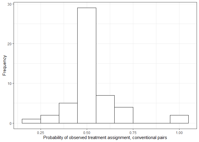
#> [6,] 0.7435420 0.5721800 0.6045299 0.8254281 0.9474680 0.0000000Using covariates \(\mathbf{X}\), we form two sets of \(50\) matched pairs, one set formed without using the dose assignment discrepancy caliper, and the other set formed using the caliper, setting the associated hyperparameters \(\xi = 0.1\) and \(M = 10000\)
# forming a set of matched pairs using conventional non-bipartite matching
pairs_vanilla <- nbp.caliper(treatment, covariates)

# forming a set of matched pairs using the dose assignment discrepancy caliper
pairs_caliper <- nbp.caliper(treatment, covariates, pmat, xi = 0.1, M = 10000)

# preview of what the pairs dataframe looks like. Contains indeces of observations,
# each row representing a matched pair
head(pairs_vanilla)
#>   High Low
#> 3    3  17
#> 4    4  65
#> 5    5  76
#> 6    6  42
#> 7    7  79
#> 8    8  28
Matched pairs formed without using the dose assignment discrepancy caliper may have probabilities of observed treatment assignment heavily deviate from \(0.5\), as shown in the plot below.
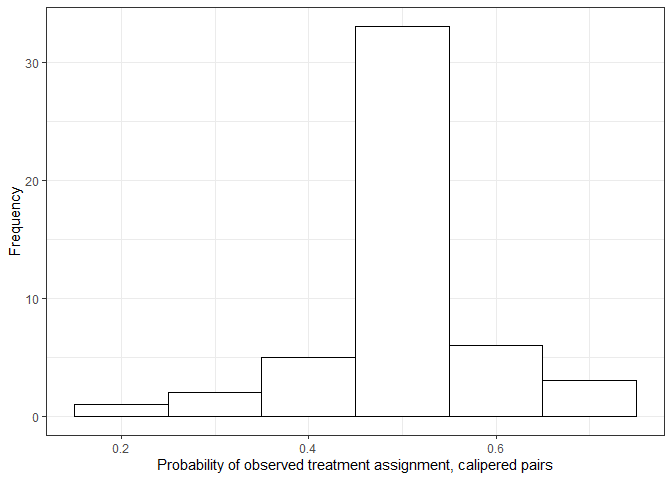
 By implementing the dose assignment discrepancy caliper and setting
\(M\) to be a large number, pairs of
observations with probability of observed treatment assignment highly
deviate from \(0.5\) are discouraged
from being formed as matched pairs.
By implementing the dose assignment discrepancy caliper and setting
\(M\) to be a large number, pairs of
observations with probability of observed treatment assignment highly
deviate from \(0.5\) are discouraged
from being formed as matched pairs.
 After forming matched pairs, we can estimate the sample average
treatment effect, either using the conventional Neyman estimator
(Baiocchi et al. 2010; Zhang et al. 2022; Heng et al. 2023) or the
bias-corrected neyman estimator (Frazier, Heng, and Zhou 2024).
After forming matched pairs, we can estimate the sample average
treatment effect, either using the conventional Neyman estimator
(Baiocchi et al. 2010; Zhang et al. 2022; Heng et al. 2023) or the
bias-corrected neyman estimator (Frazier, Heng, and Zhou 2024).
# setting "outcome" to Y
outcome <- example_data[, 2]

# Conventional Neyman estimation of sample average treatment effect
classic_estimation <- classic.neyman(outcome, treatment, pairs_vanilla)

# bias-corrected Neyman estimation of sample average treatment effect
bc_estimation <- bias.corrected.neyman(outcome, treatment, pairs_caliper, pmat, 0.1)

# displaying estimated sample average treatment effects
c(classic_estimation, bc_estimation)
#> [1] 1.969861 1.340177
Finally, a Wald-type confidence interval can be created for containing the sample average treatment effect.
# conservative variance estimation with covariate adjustment
var_est <- covAdj.variance(outcome, treatment, covariates, pairs_caliper, pmat, 0.1)

# creating a 95 percent confidence interval using the bias-corrected estimator
CI <- c(bc_estimation - qnorm(0.975)*sqrt(var_est), bc_estimation + qnorm(0.975)*sqrt(var_est))

# displaying confidence interval
CI
#> [1] -0.5952437  3.2755984