
![]()
rlandfire provides access to a diverse suite of spatial
data layers via the LANDFIRE Product Services (LFPS)
API. LANDFIRE is a joint program of
the USFS, DOI, and other major partners, which provides data layers for
wildfire management, fuel modeling, ecology, natural resource
management, climate, conservation, etc. The complete list of available
layers and additional resources can be found on the LANDFIRE
webpage.
Install rlandfire from CRAN:
install.packages("rlandfire")The development version of rlandfire can be installed
from GitHub with:
# install.packages("devtools")
devtools::install_github("bcknr/rlandfire")
Set build_vignettes = TRUE to access this vignette in
R:
devtools::install_github("bcknr/rlandfire", build_vignettes = TRUE)This package is still in development, and users may encounter bugs or unexpected behavior. Please report any issues, feature requests, or suggestions in the package’s GitHub repo.
rlandfireTo demonstrate rlandfire, we will explore how ponderosa
pine forest canopy cover changed after the 2020 Calwood fire near
Boulder, Colorado.
library(rlandfire)
library(sf)
library(terra)
library(foreign)
First, we will load the Calwood Fire perimeter data which was downloaded from Boulder County’s geospatial data hub.
boundary_file <- file.path(tempdir(), "wildfire")
utils::unzip(system.file("extdata/wildfire.zip", package = "rlandfire"),
             exdir = tempdir())

boundary <- st_read(file.path(boundary_file, "wildfire.shp")) %>%
  sf::st_transform(crs = st_crs(32613))
#> Reading layer `wildfire' from data source `/tmp/RtmpV4trFT/wildfire/wildfire.shp' using driver `ESRI Shapefile'
#> Simple feature collection with 1 feature and 7 fields
#> Geometry type: MULTIPOLYGON
#> Dimension:     XY
#> Bounding box:  xmin: -105.3901 ymin: 40.12149 xmax: -105.2471 ymax: 40.18701
#> Geodetic CRS:  WGS 84

plot(boundary$geometry, main = "Calwood Fire Boundary (2020)",
     border = "red", lwd = 1.5)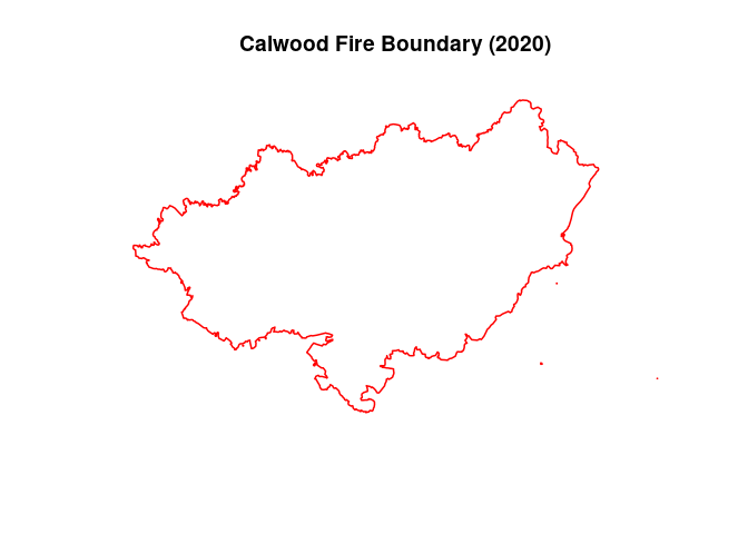
We can use the function rlandfire::getAOI() to create an
area of interest (AOI) vector with the correct format for
landfireAPIv2(). getAOI() handles several
steps for us, it ensures that the AOI is returned in the correct order
(xmin, ymin, xmax,
ymax) and converts the AOI to latitude and longitude
coordinates (as required by the API) if needed.
Using the extend argument, we will increase the AOI by 1
km in all directions to provide additional context surrounding the
burned area. This argument takes an optional numeric vector of 1, 2, or
4 elements.
aoi <- getAOI(boundary, extend = 1000)
aoi
#> [1] -105.40207   40.11224 -105.23526   40.19613
Alternatively, you can supply a LANDFIRE map zone number in place of
the AOI vector. The function getZone() returns the zone
number containing an sf object or which corresponds to the
supplied zone name. See help("getZone") for more
information and an example.
For this example, we are interested in canopy cover data for two
years, 2019 (200CC_19) and 2022 (220CC_22),
and existing vegetation type (200EVT). All available data
products, and their abbreviated names, can be found in the products table which can be
opened by calling viewProducts().
products <- c("200CC_19", "220CC_22", "200EVT")email <- "rlandfire@example.com"We can ask the API to project the data to the same CRS as our fire
perimeter data by providing the WKID for our CRS of
interest and a resolution of our choosing, in meters.
projection <- 32613
resolution <- 90We will use the edit_rule argument to filter out canopy
cover data that does not correspond to Ponderosa Pine Woodland. The
edit_rule statement should tell the API that when existing
vegetation cover is anything other than Ponderosa Pine Woodland
(7054), the value of the canopy cover layers should be set
to a specified value.
To do so, we specify that when 220EVT is not equal
(ne) to 7054, the “condition,” the canopy
cover layers should be set equal (st) to 1,
the “change.” The edit rule syntax is explained in more depth in the LFPS
guide.
(How the API applies edit rules can be unintuitive. For example,
if we used ‘clear value’ [cv] or set the value outside of
0-100 the edits we want would not work. To work around this behavior, we
set the values to 1 since it is not found in the original
data set.)
edit_rule <- list(c("condition","200EVT","ne",7054),
                  c("change", "200CC_19", "st", 1),
                  c("change", "220CC_22", "st", 1))
Note: Edits are performed in the order that they are listed and are limited to fuel theme products (i.e., Fire Behavior Fuel Model 13, Fire Behavior Fuel Model 40, Forest Canopy Base Height, Forest Canopy Bulk Density, Forest Canopy Cover, and Forest Canopy Height).
If we wanted to restrict these edits to a certain area we could pass
the path to a zip archive (.zip) containing a shapefile to
edit_mask:
edit_mask <- "path/to/wildfire.zip"Note: The file must follow ESRI shapefile naming standards (e.g., no special characters) and be less than 1MB in size.
Finally, we will provide a path to a temporary zip file. Setting the
path as a temp file is not strictly necessary because if
path is left blank landfireAPIv2() will save
the data to a temporary folder by default.
path <- tempfile(fileext = ".zip")landfireAPIv2()Now we are able to submit a request to the LANDFIRE Product Services
API with the landfireAPIv2() function.
resp <- landfireAPIv2(products = products,
                    aoi = aoi,
                    email = email,
                    projection = projection,
                    resolution = resolution,
                    edit_rule = edit_rule,
                    path = path,
                    verbose = FALSE)
landfireAPIv2() will download your requested data into
the folder provided in the path argument. If you did not provide one,
you can find the path to your data in the $path element of
the landfire_api object.
resp$pathThe files returned by the LFPS API are compressed .zip
files. We need to unzip the directory before reading the
.tif file. Note: all additional metadata is included in
this same directory.
lf_dir <- file.path(tempdir(), "lf")
utils::unzip(path, exdir = lf_dir)

lf <- terra::rast(list.files(lf_dir, pattern = ".tif$",
                             full.names = TRUE,
                             recursive = TRUE))
Now we can reclassify the canopy cover layers to remove any values which are not classified as Ponderosa Pine, calculate the change, and plot our results.
lf$US_200CC_19[lf$US_200CC_19 == 1] <- NA
lf$US_220CC_22[lf$US_220CC_22 == 1] <- NA

change <- lf$US_220CC_22 - lf$US_200CC_19

plot(change, col = rev(terrain.colors(250)),
     main = "Canopy Cover Loss - Calwood Fire (2020)",
     xlab = "Easting",
     ylab = "Northing")
plot(boundary$geometry, add = TRUE, col = NA,
     border = "black", lwd = 2)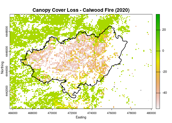
The LFPS REST API now embeds attributes in the GeoTIFF files for some
variables and returns a database file (.dbf) containing the
full attribute table.
To demonstrate, we will download the Existing Vegetation Cover
product from LF 2.4.0 (240EVC). Unlike in the example above
we will submit a minimal request with the default projection and
resolution. We will also allow rlandfire to save the files
to a temporary directory automatically. As mentioned above, we can find
the path to the temporary directory in the $path element of
the landfire_api object returned by
landfireAPIv2().
resp <- landfireAPIv2(products = "240EVC",
                    aoi = aoi,
                    email = email,
                    verbose = FALSE)
When we read in and plot the EVC layer the legend will now list the
classnames for each vegetation type.
lf_cat <- file.path(tempdir(), "lf_cat")
utils::unzip(resp$path, exdir = lf_cat)

evc <- terra::rast(list.files(lf_cat, pattern = ".tif$",
                             full.names = TRUE,
                             recursive = TRUE))

plot(evc)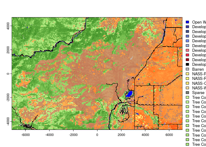
To access the values each classname is assigned to we
can uses the levels() function. This returns a simple two
column data frame containing both the index and active category, in our
case the vegetation cover classes.
head(levels(evc)[[1]])
#>   Value                        CLASSNAMES
#> 1    11                        Open Water
#> 2    13 Developed-Upland Deciduous Forest
#> 3    14 Developed-Upland Evergreen Forest
#> 4    15     Developed-Upland Mixed Forest
#> 5    16       Developed-Upland Herbaceous
#> 6    17        Developed-Upland Shrubland
Alternatively, we can access the full attribute table using two
methods. We can use the function cats() which works
similarly to levels() but returns the full attribute table
as a data frame. Alternatively, we can read the database file using
foreign::read.dbf(). Both methods return similar results,
although in this case, we see that the .dbf file includes
an additional Count column not included in the data frame
returned from cats().
# cats
attr_tbl <- cats(evc)

# Find path to database file
dbf <- list.files(lf_cat, pattern = ".dbf$",
                  full.names = TRUE,
                  recursive = TRUE)

# Read file
dbf_tbl  <- foreign::read.dbf(dbf)

head(attr_tbl[[1]])
#>   Value                        CLASSNAMES Count   R   G   B RED GREEN BLUE
#> 1    11                        Open Water   229   0   0 255   0     0  255
#> 2    13 Developed-Upland Deciduous Forest   119  64  61 168  64    61  168
#> 3    14 Developed-Upland Evergreen Forest   337  68  79 137  68    79  137
#> 4    15     Developed-Upland Mixed Forest   198 102 119 205 102   119  205
#> 5    16       Developed-Upland Herbaceous   365 122 142 245 122   142  245
#> 6    17        Developed-Upland Shrubland   181 158 170 215 158   170  215
head(dbf_tbl)
#>   Value Count                        CLASSNAMES   R   G   B      RED    GREEN
#> 1    11   229                        Open Water   0   0 255 0.000000 0.000000
#> 2    13   119 Developed-Upland Deciduous Forest  64  61 168 0.250980 0.239216
#> 3    14   337 Developed-Upland Evergreen Forest  68  79 137 0.266667 0.309804
#> 4    15   198     Developed-Upland Mixed Forest 102 119 205 0.400000 0.466667
#> 5    16   365       Developed-Upland Herbaceous 122 142 245 0.478431 0.556863
#> 6    17   181        Developed-Upland Shrubland 158 170 215 0.619608 0.666667
#>       BLUE
#> 1 1.000000
#> 2 0.658824
#> 3 0.537255
#> 4 0.803922
#> 5 0.960784
#> 6 0.843137Visit the LANDFIRE
webpage for information on citing LANDFIRE data layers. The package
citation information can be viewed with
citation("rlandfire").