![]()
Meixi Chen, Martin Lysy, Reza Ramezan
A fast Bayesian inference method for spatial random effects modelling of weather extremes. The latent spatial variables are efficiently marginalized by a Laplace approximation using the TMB library, which leverages efficient automatic differentiation in C++. The models are compiled in C++, whereas the optimization step is carried out in R. With this package, users can fit spatial GEV models with different complexities to their dataset without having to formulate the model using C++. This package also offers a method to sample from the approximate posterior distributions of both fixed and random effects, which will be useful for downstream analysis.
Before installing SpatialGEV, make sure you have TMB installed following the instructions here.
SpatialGEV uses several functions from the
INLA package for SPDE approximation to the
Matérn covariance as well as mesh creation on the spatial domain. If the
user would like to use the SPDE method (i.e. kernel="spde"
in spatialGEV_fit()), please first install package
INLA. Since INLA is
not on CRAN, it needs to be downloaded following their instruction here.
To download the stable version of this package, run
install.packages("SpatialGEV")To download the development version of this package, run
devtools::install_github("meixichen/SpatialGEV")Using the simulated data set simulatedData2 provided in
the package, we demonstrate how to use this package. Spatial variation
of the GEV parameters are plotted below.
library(SpatialGEV)
# GEV parameters simulated from Gaussian random fields
a <- simulatedData2$a # location
logb <- simulatedData2$logb # log scale
logs <- simulatedData2$logs # log shape
locs <- simulatedData2$locs # coordinate matrix
n_loc <- nrow(locs) # number of locations
y <- Map(evd::rgev, n=sample(50:70, n_loc, replace=TRUE),
         loc=a, scale=exp(logb), shape=exp(logs)) # observations

filled.contour(unique(locs$x), unique(locs$y), matrix(a, ncol=sqrt(n_loc)),
               color.palette = terrain.colors, xlab="Longitude", ylab="Latitude",
               main="Spatial variation of a",
               cex.lab=1,cex.axis=1)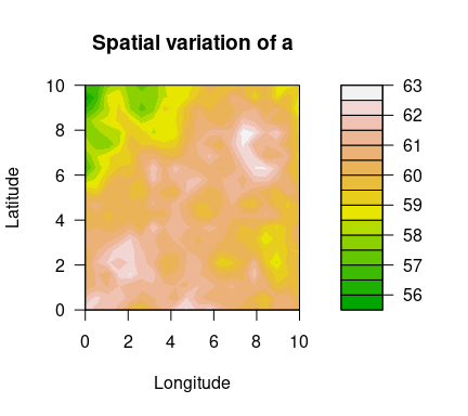
filled.contour(unique(locs$x), unique(locs$y), matrix(exp(logb), ncol=sqrt(n_loc)),
               color.palette = terrain.colors, xlab="Longitude", ylab="Latitude",
               main="Spatial variation of b",
               cex.lab=1,cex.axis=1)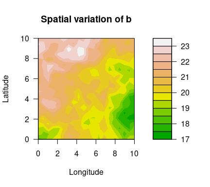
filled.contour(unique(locs$x), unique(locs$y), matrix(exp(logs), ncol=sqrt(n_loc)),
               color.palette = terrain.colors, xlab="Longitude", ylab="Latitude",
               main="Spatial variation of s",
               cex.lab=1,cex.axis=1)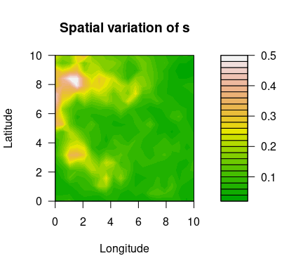
To fit a GEV-GP model to the simulated data, use the
spatialGEV_fit() function. We use random="abs"
to indicate that all three GEV parameters are treated as random effects.
The shape parameter s is constrained to be positive (log
transformed) by specifying reparam_s="positive". The
covariance kernel function used here is the SPDE-approximated Matérn
kernel kernel="spde". Initial parameter values are passed
to init_param using a list.
fit <- spatialGEV_fit(data = y, locs = locs, random = "abs",
                      init_param = list(a = rep(60, n_loc),
                                        log_b = rep(2,n_loc),
                                        s = rep(-3,n_loc),
                                        beta_a = 60, beta_b = 2, beta_s = -2,
                                        log_sigma_a = 1.5, log_kappa_a = -2,
                                        log_sigma_b = 1.5, log_kappa_b = -2,
                                        log_sigma_s = -1, log_kappa_s = -2),
                      reparam_s = "positive", kernel="spde", silent = TRUE)

class(fit)
#> [1] "spatialGEVfit"
print(fit)
#> Model fitting took 27.9517922401428 seconds
#> The model has reached relative convergence
#> The model uses a spde kernel
#> Number of fixed effects in the model is 9
#> Number of random effects in the model is 1308
#> Hessian matrix is positive definite. Use spatialGEV_sample to obtain posterior samples
Posterior samples of the random and fixed effects are drawn using
spatialGEV_sample(). Specify observation=TRUE
if we would also like to draw from the posterior predictive
distribution.
sam <- spatialGEV_sample(model = fit, n_draw = 1000, observation = T)
print(sam)
#> The samples contains 1000 draws of 1209 parameters
#> The samples contains 1000 draws of response at 400 locations
#> Use summary() to obtain summary statistics of the samples
To get summary statistics of the posterior samples, use
summary() on the sample object.
pos_summary <- summary(sam)
pos_summary$param_summary[1:5,]
#>        2.5%      25%      50%      75%    97.5%     mean
#> a1 59.98220 61.58412 62.39717 63.23451 64.98185 62.40852
#> a2 60.39339 61.75672 62.55552 63.30514 64.95137 62.55192
#> a3 60.01955 61.28410 61.98922 62.71080 64.13772 61.98618
#> a4 59.57800 60.92354 61.66539 62.39592 63.81774 61.66007
#> a5 59.55668 60.86209 61.54278 62.21564 63.68217 61.55340
pos_summary$y_summary[1:5,]
#>        2.5%      25%      50%      75%    97.5%     mean
#> y1 39.43693 56.12927 70.41943 87.22232 140.3342 74.81315
#> y2 37.09989 55.68274 67.98861 87.42057 148.5369 74.42377
#> y3 38.46096 55.07948 69.19833 87.29214 152.6150 74.99553
#> y4 38.34585 56.38710 68.56856 86.17946 143.4025 73.64138
#> y5 37.81648 55.14434 69.23200 85.81161 143.7851 74.12148
Consider a shorter name, e.g., sgev_*, than
spatialGEV_*.
Argument init_params adds a lot of complexity to
spatialGEV_fit(). Perhaps this function can be broken down
into two parts: spatialGEV_adfun() which returns the
adfun object, and then spatialGEV_fit() which
does the fitting. The advantage is that the
adfun$env$parameters object tells you the dimension of the
parameter values, which can be useful for initialization. Also, note
that adfun$env$data object contains the entire data list
for browsing.
Write some tests for the spde kernel. Construct the sparse
precision matrix using get_spde_prec(), invert it using
Matrix::solve(), apply the scale factor, and pass as
variance to dmvnorm().